Thursday, 9 May 2013

12. Define discrete Fourier transform and its inverse.


>Table of contents

The discrete Fourier transform pair that applies to sampled function is given by,

For u = 0, 1, 2 . . . . , N-1, and

For x = 0, 1, 2 . . . ., N-1.

In the two variable case the discrete Fourier transform pair is

For u = 0, 1, 2 . . . , M-1, v = 0, 1, 2 . . . , N - 1, and

For x = 0, 1, 2 . . . , M-1, y = 0, 1, 2 . . . , N-1.

If M = N, then discrete Fourier transform pair is


For u, v = 0, 1, 2 . . . , N – 1, and

For x, y = 0, 1, 2 . . . , N – 1


>Table of contents


Thursday, 2 May 2013

11. Define Fourier Transform and its inverse.


>Table of contents

Let f(x) be a continuous function of a real variable x. The Fourier transform of f(x) is
defined by the equation

Where j = √-1

Given F(u), f(x) can be obtained by using the inverse Fourier transform
The Fourier transform exists if f(x) is continuous and integrable and F(u) is integrable.

The Fourier transform of a real function, is generally complex,

                                                      F(u) = R(u) + jI(u)

Where R(u) and I(u) are the real and imaginary components of F(u). F(u) can be expressed in
exponential form as

                                                      F(u) = │F(u)│ejØ(u)

where
                                                    │F(u)│ = [R2(u) + I2(u)]1/2

and
                                               Ø (u, v) = tan-1[ I (u, v)/R (u, v) ]

The magnitude function |F (u)| is called the Fourier Spectrum of f(x) and Φ(u) its phase angle.
The variable u appearing in the Fourier transform is called the frequency variable.

                                           Fig 1 A simple function and its Fourier spectrum

 The Fourier transform can be easily extended to a function f(x, y) of two variables. If f(x, y) is
continuous and integrable and F(u,v) is integrable, following Fourier transform pair exists

 and


 Where u, v are the frequency variables

 The Fourier spectrum, phase, are

                                                    |F(u, v)|  = [R2(u, v) + I2(u, v )]1/2

                                                        Ø(u, v) = tan-1[ I(u, v)/R(u, v) ]


>Table of contents


Tuesday, 30 April 2013

10. Write about perspective image transformation.


>Table of contents
 
A perspective transformation (also called an imaging transformation) projects 3D points onto a
plane. Perspective transformations play a central role in image processing because they provide
an approximation to the manner in which an image is formed by viewing a 3D world. These
transformations are fundamentally different, because they are nonlinear in that they involve
division by coordinate values.

Figure 10 shows a model of the image formation process. The camera coordinate system (x, y, z)
has the image plane coincident with the xy plane and the optical axis (established by the center
of the lens) along the z axis. Thus the center of the image plane is at the origin, and the centre of
the lens is at coordinates (0.0, λ). If the camera is in focus for distant objects, λ is the focal length
of the lens. Here the assumption is that the camera coordinate system is aligned with the world
coordinate system (X, Y, Z).

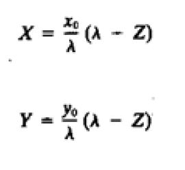
Let (X,Y,Z) be the world co-ordinates of any point in a 3-D scene, as shown in the Fig 10. We assume throughout the following discussion that Z>λ ; that is all points of interest lie in front of the lens.The first step is to obtain a relationship that gives the coordinates (x,y) of the projection of the point (X,Y,Z) onto the image plane.This is easily accomplished by the use of similar triangles. With reference to Fig 10,

Fig 10 Basic model of the imaging process The camera coordinate system (x, y, z) is aligned with the world coordinate system (X, Y, Z)


 Where the negative signs in front of X and Y indicate that image points are actually inverted, as the geometry of Fig 10 shows.
The image-plane coordinates of the projected 3-D point follow directly from above equations
These equations are nonlinear because they involve division by the variable Z. Although we could use them directly as shown, it is often convenient to express them in linear matrix form, for rotation, translation and scaling. This is easily accomplished by dividing the first three homogeneous coordinates by the fourth. A point in the cartesian world coordinate system may be expressed in vector form as
and its homogeneous counterpart is
If we define the perspective transformation matrix as
The product PWh yields a vector denoted Ch
                                                                             Ch=PWh


The element of ch is the camera coordinates in homogeneous form. As indicated, these
coordinates can be converted to Cartesian form by dividing each of the first three components of
ch by the fourth. Thus the Cartesian of any point in the camera coordinate system are given in
vector form by

 The first two components of c are the (x, y) coordinates in the image plane of a projected 3-D
point (X, Y, Z). The third component is of no interest in terms of the model in Fig. 10. As shown
next, this component acts as a free variable in the inverse perspective transformation

 The inverse perspective transformation maps an image point back into 3-D.
 wh=P-1Ch
 Where P-1 is  

 Suppose that an image point has coordinates (xo, yo, 0), where the 0 in the z location simply
indicates that the image plane is located at z = 0. This point may be expressed in homogeneous
vector form as
 or, in Cartesian coordinates

 This result obviously is unexpected because it gives Z = 0 for any 3-D point. The problem here is
caused by mapping a 3-D scene onto the image plane, which is a many-to-one transformation.
The image point (x0, y0) corresponds to the set of collinear 3-D points that lie on the line passing
through (xo, yo, 0) and (0, 0, λ). The equation of this line in the world coordinate system; that is,

Equations above show that unless something is known about the 3-D point that generated an
image point (for example, its Z coordinate) it is not possible to completely recover the 3-D point
from its image. This observation, which certainly is not unexpected, can be used to formulate the
inverse perspective transformation by using the z component of ch as a free variable instead of 0.
Thus, by letting
It thus follows


 which upon conversion to Cartesian coordinate gives
 In other words, treating z as a free variable yields the equations

 Solving for z in terms of Z in the last equation and substituting in the first two expressions yields

 which agrees with the observation that revering a 3-D point from its image by means of the
inverse perspective transformation requires knowledge of at least one of the world coordinates of
the point.


>Table of contents

9. Explain about the basic relationships and distance measures between pixels in a digital image.


>Table of contents
 
Neighbors of a Pixel:

A pixel p at coordinates (x, y) has four horizontal and vertical neighbors whose coordinates are
given by (x+1, y), (x-1, y), (x, y+1), (x, y-1). This set of pixels, called the 4-neighbors of p, is
denoted by N4 (p). Each pixel is a unit distance from (x, y), and some of the neighbors of p lie
outside the digital image if (x, y) is on the border of the image.

The four diagonal neighbors of p have coordinates (x+1, y+1), (x+1, y-1), (x-1, y+1), (x-1, y-1)
and are denoted by ND (p). These points, together with the 4-neighbors, are called the 8-
neighbors of p, denoted by N8 (p). As before, some of the points in ND (p) and N8 (p) fall outside
the image if (x, y) is on the border of the image.

Connectivity:

Connectivity between pixels is a fundamental concept that simplifies the definition of numerous
digital image concepts, such as regions and boundaries. To establish if two pixels are connected,
it must be determined if they are neighbors and if their gray levels satisfy a specified criterion of
similarity (say, if their gray levels are equal). For instance, in a binary image with values 0 and 1,
two pixels may be 4-neighbors, but they are said to be connected only if they have the same
value.

Let V be the set of gray-level values used to define adjacency. In a binary image, V={1} if we
are referring to adjacency of pixels with value 1. In a grayscale image, the idea is the same, but
set V typically contains more elements. For example, in the adjacency of pixels with a range of
possible gray-level values 0 to 255, set V could be any subset of these 256 values. We consider
three types of adjacency:

(a) 4-adjacency. Two pixels p and q with values from V are 4-adjacent if q is in the set N4 (p).

(b) 8-adjacency. Two pixels p and q with values from V are 8-adjacent if q is in the set N8 (p).

(c) m-adjacency (mixed adjacency).Two pixels p and q with values from V are m-adjacent if

(i) q is in N4 (p), or

(ii) q is in ND (p) and the set has no pixels whose values are from V.

Mixed adjacency is a modification of 8-adjacency. It is introduced to eliminate the ambiguities
that often arise when 8-adjacency is used. For example, consider the pixel arrangement shown in
Fig.9 (a) for V= {1}.The three pixels at the top of Fig.9 (b) show multiple (ambiguous) 8-
adjacency, as indicated by the dashed lines. This ambiguity is removed by using m-adjacency, as
shown in Fig. 9 (c).Two image subsets S1 and S2 are adjacent if some pixel in S1 is adjacent to
some pixel in S2. It is understood here and in the following definitions that adjacent means 4-, 8-
, or m-adjacent. A (digital) path (or curve) from pixel p with coordinates (x, y) to pixel q with
coordinates (s, t) is a sequence of distinct pixels with coordinates
                     (x0,y0),(x1,y1),.............................................................,(xn,yn)
where (x0,y0)=(x,y) and (xn,yn)=(s,t) and pixels (xiyi) and  (xi-1,yi-1) are adjacent for 1<=i<=n.
In this case, n is the length of the path. If (x0, y0) = (xn, yn) , the path is a closed path. We can define 4-, 8-, or m-paths depending on the type of adjacency specified. For example, the paths shown in Fig. 9 (b) between the northeast and southeast points are 8-paths, and the path in Fig. 9 (c) is an m-path. Note the absence of ambiguity in the m-path. Let S represent a subset of pixels in an image. Two pixels p and q are said to be connected in S if there exists a path between them consisting entirely of pixels in S. For any pixel p in S, the set of pixels that are connected to it in S is called a connected component of S. If it only has one connected component, then set S is called a connected set.

Let R be a subset of pixels in an image. We call R a region of the image if R is a connected set.
The boundary (also called border or contour) of a region R is the set of pixels in the region that
have one or more neighbors that are not in R. If R happens to be an entire image (which we
recall is a rectangular set of pixels), then its boundary is defined as the set of pixels in the first
and last rows and columns of the image. This extra definition is required because an image has
no neighbors beyond its border. Normally, when we refer to a region, we are referring to a subset
Fig.9 (a) Arrangement of pixels; (b) pixels that are 8-adjacent (shown dashed) to the center
pixel; (c) m-adjacency

of an image, and any pixels in the boundary of the region that happen to coincide with the border
of the image are included implicitly as part of the region boundary.

Distance Measures:

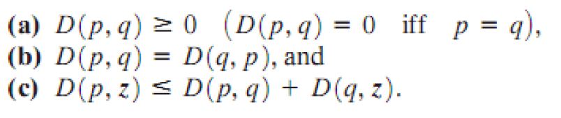
For pixels p, q, and z, with coordinates (x, y), (s, t), and (v, w), respectively, D is a distance
function or metric if

 The Euclidean distance between p and q is defined as
 For this distance measure, the pixels having a distance less than or equal to some value r from(x,
y) are the points contained in a disk of radius r centered at (x, y).

 The D4 distance (also called city-block distance) between p and q is defined as
 In this case, the pixels having a D4 distance from (x, y) less than or equal to some value r form a
diamond centered at (x, y). For example, the pixels with D4 distance . 2 from (x, y) (the center
point) form the following contours of constant distance:

The pixels with D4 =1 are the 4-neighbors of (x, y).

 The D8 distance (also called chessboard distance) between p and q is defined as
 In this case, the pixels with D8 distance from(x, y) less than or equal to some value r form a
square centered at (x, y). For example, the pixels with D8 distance ≤ 2 from(x, y) (the center
point) form the following contours of constant distance:

 The pixels with D8=1 are the 8-neighbors of (x, y). Note that the D4 and D8 distances between p
and q are independent of any paths that might exist between the points because these distances
involve only the coordinates of the points. If we elect to consider m-adjacency, however, the Dm
distance between two points is defined as the shortest m-path between the points. In this case, the
distance between two pixels will depend on the values of the pixels along the path, as well as the
values of their neighbors. For instance, consider the following arrangement of pixels and assume
that p, p2 , and p4 have value 1 and that p1 and p3 can have a value of 0 or 1:
 Suppose that we consider adjacency of pixels valued 1 (i.e. = {1}). If p1 and p3 are 0, the length
of the shortest m-path (the Dm distance) between p and p4 is 2. If p1 is 1, then p2 and p will no
longer be m-adjacent (see the definition of m-adjacency) and the length of the shortest m-path
becomes 3 (the path goes through the points pp1p2p4). Similar comments apply if p3 is 1 (and p1
is 0); in this case, the length of the shortest m-path also is 3. Finally, if both p1 and p3 are 1 the
length of the shortest m-path between p and p4 is 4. In this case, the path goes through the
sequence of points pp1p2p3p4.

>Table of contents

Saturday, 27 April 2013

8. Explain about Aliasing and Moire patterns.


>Table of contents

Aliasing and Moiré Patterns:

Functions whose area under the curve is finite can be represented in terms of sines and cosines of
various frequencies. The sine/cosine component with the highest frequency determines the
highest “frequency content” of the function. Suppose that this highest frequency is finite and that
the function is of unlimited duration (these functions are called band-limited functions).Then, the
Shannon sampling theorem [Brace well (1995)] tells us that, if the function is sampled at a rate
equal to or greater than twice its highest frequency, it is possible to recover completely the
original function from its samples. If the function is undersampled, then a phenomenon called
aliasing corrupts the sampled image. The corruption is in the form of additional frequency
components being introduced into the sampled function. These are called aliased frequencies.
Note that the sampling rate in images is the number of samples taken (in both spatial directions)
per unit distance.

As it turns out, except for a special case discussed in the following paragraph, it is impossible to
satisfy the sampling theorem in practice. We can only work with sampled data that are finite in
duration. We can model the process of converting a function of unlimited duration into a
function of finite duration simply by multiplying the unlimited function by a “gating function”
that is valued 1 for some interval and 0 elsewhere. Unfortunately, this function itself has
frequency components that extend to infinity. Thus, the very act of limiting the duration of a
band-limited function causes it to cease being band limited, which causes it to violate the key
condition of the sampling theorem. The principal approach for reducing the aliasing effects on an
image is to reduce its high-frequency components by blurring the image prior to sampling.
However, aliasing is always present in a sampled image. The effect of aliased frequencies can be
seen under the right conditions in the form of so called Moiré patterns.

There is one special case of significant importance in which a function of infinite duration can be
sampled over a finite interval without violating the sampling theorem. When a function is
periodic, it may be sampled at a rate equal to or exceeding twice its highest frequency and it is
possible to recover the function from its samples provided that the sampling captures exactly an
integer number of periods of the function. This special case allows us to illustrate vividly the
Moiré effect. Figure 8 shows two identical periodic patterns of equally spaced vertical bars,
rotated in opposite directions and then superimposed on each other by multiplying the two
images. A Moiré pattern, caused by a breakup of the periodicity, is seen in Fig.8 as a 2-D
sinusoidal (aliased) waveform (which looks like a corrugated tin roof) running in a vertical
direction. A similar pattern can appear when images are digitized (e.g., scanned) from a printed
page, which consists of periodic ink dots.

                                             Fig.8. Illustration of the Moiré pattern effect


>Table of contents


Wednesday, 10 April 2013

7. Define spatial and gray level resolution. Explain about isopreference curves.


>Table of contents


Spatial and Gray-Level Resolution:

Sampling is the principal factor determining the spatial resolution of an image. Basically, spatial
resolution is the smallest discernible detail in an image. Suppose that we construct a chart with
vertical lines of width W, with the space between the lines also having width W.A line pair
consists of one such line and its adjacent space. Thus, the width of a line pair is 2W, and there
are 1/2Wline pairs per unit distance. A widely used definition of resolution is simply the smallest
number of discernible line pairs per unit distance; for example, 100 line pairs per millimeter.
Gray-level resolution similarly refers to the smallest discernible change in gray level. We have
considerable discretion regarding the number of samples used to generate a digital image, but
this is not true for the number of gray levels. Due to hardware considerations, the number of gray
levels is usually an integer power of 2.

The most common number is 8 bits, with 16 bits being used in some applications where
enhancement of specific gray-level ranges is necessary. Sometimes we find systems that can
digitize the gray levels of an image with 10 or 12 bit of accuracy, but these are the exception
rather than the rule. When an actual measure of physical resolution relating pixels and the level
of detail they resolve in the original scene are not necessary, it is not uncommon to refer to an Llevel
digital image of size M*N as having a spatial resolution of M*N pixels and a gray-level
resolution of L levels.


Fig.7.1. A 1024*1024, 8-bit image subsampled down to size 32*32 pixels The number of
allowable gray levels was kept at 256.

The subsampling was accomplished by deleting the appropriate number of rows and columns
from the original image. For example, the 512*512 image was obtained by deleting every other
row and column from the 1024*1024 image. The 256*256 image was generated by deleting
every other row and column in the 512*512 image, and so on. The number of allowed gray
levels was kept at 256. These images show the dimensional proportions between various
sampling densities, but their size differences make it difficult to see the effects resulting from a
reduction in the number of samples. The simplest way to compare these effects is to bring all the
subsampled images up to size 1024*1024 by row and column pixel replication. The results are
shown in Figs. 7.2 (b) through (f). Figure7.2 (a) is the same 1024*1024, 256-level image shown
in Fig.7.1; it is repeated to facilitate comparisons.

Fig. 7.2 (a) 1024*1024, 8-bit image (b) 512*512 image resampled into 1024*1024 pixels by
row and column duplication (c) through (f) 256*256, 128*128, 64*64, and 32*32 images
resampled into 1024*1024 pixels

Compare Fig. 7.2(a) with the 512*512 image in Fig. 7.2(b) and note that it is virtually impossible
to tell these two images apart. The level of detail lost is simply too fine to be seen on the printed
page at the scale in which these images are shown. Next, the 256*256 image in Fig. 7.2(c) shows
a very slight fine checkerboard pattern in the borders between flower petals and the black background.A slightly more pronounced graininess throughout the image also is beginning to appear.
These effects are much more visible in the 128*128 image in Fig. 7.2(d), and they become
pronounced in the 64*64 and 32*32 images in Figs. 7.2 (e) and (f), respectively.

In the next example, we keep the number of samples constant and reduce the number of gray
levels from 256 to 2, in integer powers of 2.Figure 7.3(a) is a 452*374 CAT projection image,
displayed with k=8 (256 gray levels). Images such as this are obtained by fixing the X-ray source
in one position, thus producing a 2-D image in any desired direction. Projection images are used
as guides to set up the parameters for a CAT scanner, including tilt, number of slices, and range.
Figures 7.3(b) through (h) were obtained by reducing the number of bits from k=7 to k=1 while
keeping the spatial resolution constant at 452*374 pixels. The 256-, 128-, and 64-level images
are visually identical for all practical purposes. The 32-level image shown in Fig. 7.3 (d),
however, has an almost imperceptible set of very fine ridge like structures in areas of smooth
gray levels (particularly in the skull).This effect, caused by the use of an insufficient number of
gray levels in smooth areas of a digital image, is called false contouring, so called because the
ridges resemble topographic contours in a map. False contouring generally is quite visible in
images displayed using 16 or less uniformly spaced gray levels, as the images in Figs. 7.3(e)
through (h) show.

Fig. 7.3 (a) 452*374, 256-level image (b)–(d) Image displayed in 128, 64, and 32 gray levels,
while keeping the spatial resolution constant (e)–(g) Image displayed in 16, 8, 4, and 2 gray
levels.

As a very rough rule of thumb, and assuming powers of 2 for convenience, images of size
256*256 pixels and 64 gray levels are about the smallest images that can be expected to be
reasonably free of objectionable sampling checker-boards and false contouring.

The results in Examples 7.2 and 7.3 illustrate the effects produced on image quality by varying N
and k independently. However, these results only partially answer the question of how varying N
and k affect images because we have not considered yet any relationships that might exist
between these two parameters.

An early study by Huang [1965] attempted to quantify experimentally the effects on image
quality produced by varying N and k simultaneously. The experiment consisted of a set of
subjective tests. Images similar to those shown in Fig.7.4 were used. The woman’s face is
representative of an image with relatively little detail; the picture of the cameraman contains an
intermediate amount of detail; and the crowd picture contains, by comparison, a large amount of
detail. Sets of these three types of images were generated by varying N and k, and observers
were then asked to rank them according to their subjective quality. Results were summarized in
the form of so-called isopreference curves in the Nk-plane (Fig.7.5 shows average isopreference
curves representative of curves corresponding to the images shown in Fig. 7.4).Each point in the
Nk-plane represents an image having values of N and k equal to the coordinates of that point.

 Fig.7.4 (a) Image with a low level of detail (b) Image with a medium level of detail (c) Image
with a relatively large amount of detail

Points lying on an isopreference curve correspond to images of equal subjective quality. It was
found in the course of the experiments that the isopreference curves tended to shift right and
upward, but their shapes in each of the three image categories were similar to those shown in Fig. 7.5. This is not unexpected, since a shift up and right in the curves simply means larger values for N and k, which implies better picture quality.

Fig.7.5. Representative isopreference curves for the three types of images in Fig.7.4

The key point of interest in the context of the present discussion is that isopreference curves tend
to become more vertical as the detail in the image increases. This result suggests that for images
with a large amount of detail only a few gray levels may be needed. For example, the
isopreference curve in Fig.7.5 corresponding to the crowd is nearly vertical. This indicates that,
for a fixed value of N, the perceived quality for this type of image is nearly independent of the
number of gray levels used. It is also of interest to note that perceived quality in the other two
image categories remained the same in some intervals in which the spatial resolution was
increased, but the number of gray levels actually decreased. The most likely reason for this result
is that a decrease in k tends to increase the apparent contrast of an image, a visual effect that
humans often perceive as improved quality in an image.

>Table of contents

Monday, 11 March 2013

6. Explain about image sampling and quantization process.


>Table of contents


Image Sampling and Quantization:

The output of most sensors is a continuous voltage waveform whose amplitude and spatial
behavior are related to the physical phenomenon being sensed. To create a digital image, we
need to convert the continuous sensed data into digital form. This involves two processes:
sampling and quantization.

Basic Concepts in Sampling and Quantization:

The basic idea behind sampling and quantization is illustrated in Fig.6.1. Figure 6.1(a) shows a
continuous image, f(x, y), that we want to convert to digital form. An image may be continuous
with respect to the x- and y-coordinates, and also in amplitude. To convert it to digital form, we
have to sample the function in both coordinates and in amplitude. Digitizing the coordinate
values is called sampling. Digitizing the amplitude values is called quantization.

The one-dimensional function shown in Fig.6.1 (b) is a plot of amplitude (gray level) values of
the continuous image along the line segment AB in Fig. 6.1(a).The random variations are due to
image noise. To sample this function, we take equally spaced samples along line AB, as shown
in Fig.6.1 (c).The location of each sample is given by a vertical tick mark in the bottom part of
the figure. The samples are shown as small white squares superimposed on the function. The set
of these discrete locations gives the sampled function. However, the values of the samples still
span (vertically) a continuous range of gray-level values. In order to form a digital function, the
gray-level values also must be converted (quantized) into discrete quantities. The right side of
Fig. 6.1 (c) shows the gray-level scale divided into eight discrete levels, ranging from black to
white. The vertical tick marks indicate the specific value assigned to each of the eight gray
levels. The continuous gray levels are quantized simply by assigning one of the eight discrete
gray levels to each sample. The assignment is made depending on the vertical proximity of a
sample to a vertical tick mark. The digital samples resulting from both sampling and quantization
are shown in Fig.6.1 (d). Starting at the top of the image and carrying out this procedure line by
line produces a two-dimensional digital image.

Sampling in the manner just described assumes that we have a continuous image in both
coordinate directions as well as in amplitude. In practice, the method of sampling is determined
by the sensor arrangement used to generate the image. When an image is generated by a single sensing element combined with mechanical motion, as in Fig. 2.13, the output of the sensor is
quantized in the manner described above. However, sampling is accomplished by selecting the
number of individual mechanical increments at which we activate the sensor to collect data.
Mechanical motion can be made very exact so, in principle; there is almost no limit as to how
fine we can sample an image. However, practical limits are established by imperfections in the
optics used to focus on the sensor an illumination spot that is inconsistent with the fine resolution achievable with mechanical displacements. When a sensing strip is used for image acquisition, the number of sensors in the strip establishes the sampling limitations in one image direction. Mechanical
motion in the other direction can be controlled more accurately, but it makes little sense to try to
achieve sampling density in one direction that exceeds the sampling limits established by the
number of sensors in the other. Quantization of the sensor outputs completes the process of
generating a digital image.

Fig.6.1. Generating a digital image (a) Continuous image (b) A scan line from A to Bin the
continuous image, used to illustrate the concepts of sampling and quantization (c) Sampling
and quantization. (d) Digital scan line

When a sensing array is used for image acquisition, there is no motion and the number of sensors
in the array establishes the limits of sampling in both directions. Figure 6.2 illustrates this
concept. Figure 6.2 (a) shows a continuous image projected onto the plane of an array sensor.
Figure 6.2 (b) shows the image after sampling and quantization. Clearly, the quality of a digital
image is determined to a large degree by the number of samples and discrete gray levels used in
sampling and quantization.

Fig.6.2. (a) Continuos image projected onto a sensor array (b) Result of image
sampling and quantization.

>Table of contents