35. Explain about Ideal Low Pass Filter (ILPF) in frequency domain.

35. Explain about Ideal Low Pass Filter (ILPF) in frequency domain.

   February 27, 2014       legend

---

Lowpass Filter:

The edges and other sharp transitions (such as noise) in the gray levels of an image contribute significantly to the high-frequency content of its Fourier transform. Hence blurring (smoothing) is achieved in the frequency domain by attenuating us the transform of a given image.

G (u, v) = H (u, v) F(u, v)

where F (u, v) is the Fourier transform of an image to be smoothed. The problem is to select a filter transfer function H (u, v) that yields G (u, v) by attenuating the high-frequency components of F (u, v). The inverse transform then will yield the desired smoothed image g (x, y).

Ideal Filter:

A 2-D ideal lowpass filter (ILPF) is one whose transfer function satisfies the relation

\[H(u,v)=\begin{cases}1 & D(u,v) \leq D_{0}\\0 & D(u,v) > D_{0}\end{cases}\]

where D is a specified non negative quantity, and D(u, v) is the distance from point (u, v) to the
origin of the frequency plane; that is,
\[D(u,v)=\sqrt{(u^{2}+v^{2})}\]
Figure 3 (a) shows a 3-D perspective plot of H (u, v) u a function of u and v. The name ideal filter indicates that oil frequencies inside a circle of radius D₀ are passed with no attenuation, whereas all frequencies outside this circle are completely attenuated.

Fig.3 (a) Perspective plot of an ideal lowpass filter transfer function; (b) filter cross
section.

The lowpass filters are radially symmetric about the origin. For this type of filter, specifying a cross section extending as a function of distance from the origin along a radial line is sufficient, as Fig. 3 (b) shows. The complete filter transfer function can then be generated by rotating the cross section 360 about the origin. Specification of radially symmetric filters centered on the N x N frequency square is based on the assumption that the origin of the Fourier transform has been centered on the square.

For an ideal lowpass filter cross section, the point of transition between H(u, v) = 1 and H(u, v) = 0 is often called the cutoff frequency. In the case of Fig.3 (b), for example, the cutoff frequency is Do. As the cross section is rotated about the origin, the point Do traces a circle giving a locus of cutoff frequencies, all of which are a distance Do from the origin. The cutoff frequency concept is quite useful in specifying filter characteristics. It also serves as a common base for comparing the behavior of different types of filters.

The sharp cutoff frequencies of an ideal lowpass filter cannot be realized with electronic components, although they can certainly be simulated in a computer.

Read More

19.Define discrete cosine transform.

19.Define discrete cosine transform.

   December 28, 2013       legend

---

>Table of contents
 
 The 1-D discrete cosine transform is defined as

For u = 0, 1, 2, . . , N-1. Similarly the inverse DCT is defined as

 

For u = 0, 1, 2, . . , N-1

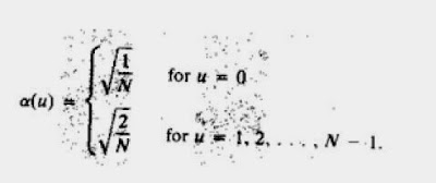
Where α is

 

 The corresponding 2-D DCT pair is

 For u, v = 0, 1, 2, . . , N-1, and

For x, y= 0, 1, 2, . . , N-1

>Table of contents
 

Read More

18.What are the properties of Slant transform?

18.What are the properties of Slant transform?

   December 28, 2013       legend

---

>Table of contents
 
 Properties of Slant transform

 (i) The slant transform is real and orthogonal.

 S = S*

 S^-1 = S^T

(ii) The slant transform is fast, it can be implemented in (N log₂N) operations on an N x 1 vector.

(iii) The energy deal for images in this transform is rated in very good to excellent range.

(iv) The mean vectors for slant transform matrix S are not sequentially ordered for n ≥ 3.

>Table of contents

Read More

17.Write about Slant transform.

17.Write about Slant transform.

   December 28, 2013       legend

---

>Table of contents
 
 The Slant transform matrix of order N x N is the recursive expression S_n is given by

 Where I_m is the identity matrix of order M x M, and

 The coefficients are

 and

 The slant transform for N = 4 will be

>Table of contents

Read More

16.Explain the basic principle of Hotelling transform.

16.Explain the basic principle of Hotelling transform.

   December 28, 2013       legend

---

>Table of contents
 
Hotelling transform:

The basic principle of hotelling transform is the statistical properties of vector
representation. Consider a population of random vectors of the form,

And the mean vector of the population is defined as the expected value of x i.e.,

m_x = E{x}

The suffix m represents that the mean is associated with the population of x vectors. The
expected value of a vector or matrix is obtained by taking the expected value of each elememt.
The covariance matrix C_x in terms of x and m_x is given as

C_x = E{(x-m_x) (x-m_x)^T} 

T denotes the transpose operation. Since, x is n dimensional, {(x-m_x) (x-m_x)^T} will be of
n x n dimension. The covariance matrix is real and symmetric. If elements xi and xj are
uncorrelated, their covariance is zero and, therefore, c_ij = c_ji = 0.

For M vector samples from a random population, the mean vector and covariance matrix
can be approximated from the samples by

 and

 

>Table of contents

 

Read More

15.State distributivity and scaling property of 2D DFT

15.State distributivity and scaling property of 2D DFT

   December 28, 2013       legend

---

>Table of contents
 
Distributivity:

From the definition of the continuous or discrete transform pair,

and, in general,

In other words, the Fourier transform and its inverse are distributive over addition but not over
multiplication.

Scaling:

For two scalars a and b,

af (x, y) <=> aF(u, v)

>Table of contents
 

Read More

14.State and prove the translation property of 2D-DFT

14.State and prove the translation property of 2D-DFT

   December 05, 2013       legend

---

 >Table of contents

The translation properties of the Fourier transform pair are

and

Where the double arrow indicates the correspondence between a function and its Fourier
Transform,
Equation (1) shows that multiplying f(x, y) by the indicated exponential term and taking
the transform of the product results in a shift of the origin of the frequency plane to the point (u_o,
v_o).

Consider the equation (1) with u_o = v_o = N/2 or
                                              exp[j2Π(u_ox + v_oy)/N] = e^{jΠ(x + y)}
                                                                                   = (-1)^{(x + y)}
and
                                          f(x, y)(-1)^x+y = F(u – N/2, v – N/2)

Thus the origin of the Fourier transform of f(x, y) can be moved to the center of its
corresponding N x N frequency square simply by multiplying f(x, y) by (-1)^x+y . In the one
variable case this shift reduces to multiplication of f(x) by the term (-1)^x. Note from equation (2)
that a shift in f(x, y) does not affect the magnitude of its Fourier transform as,

 

 >Table of contents

Read More

13.State and prove separability property of 2D-DFT.

13.State and prove separability property of 2D-DFT.

   December 05, 2013       legend

---

 >Table of contents

 The separability property of 2D-DFT states that, the discrete Fourier transform pair can
be expressed in the separable forms. i.e. ,
                                                                                                                                                             (1)

 For u, v = 0, 1, 2 . . . , N – 1, and


                                                                                                                                                             (2)

For x, y = 0, 1, 2 . . . , N – 1

The principal advantage of the separability property is that F(u,v) or f(x,y) can be
obtained in two steps by successive applications of the 1-D Fourier transform or its inverse. This
advantage becomes evident if equation (1) is expressed in the form


                                                                                                                                                         (3)

Where,

(4)

 For each value of x, the expression inside the brackets in eq(4) is a 1-D transform, with
frequency values v = 0, 1, . . . , N-1. Therefore the 2-D function f(x, v) is obtained by taking a
transform along each row of f(x, y) and multiplying the result by N. The desired result, F(u, v), is
then obtained by taking a transform along each column of F(x, v), as indicated by eq(3)

 >Table of contents

Read More

12. Define discrete Fourier transform and its inverse.

12. Define discrete Fourier transform and its inverse.

   May 09, 2013       legend

---

>Table of contents

The discrete Fourier transform pair that applies to sampled function is given by,

For u = 0, 1, 2 . . . . , N-1, and

For x = 0, 1, 2 . . . ., N-1.

In the two variable case the discrete Fourier transform pair is

For u = 0, 1, 2 . . . , M-1, v = 0, 1, 2 . . . , N - 1, and

For x = 0, 1, 2 . . . , M-1, y = 0, 1, 2 . . . , N-1.

If M = N, then discrete Fourier transform pair is

For u, v = 0, 1, 2 . . . , N – 1, and

For x, y = 0, 1, 2 . . . , N – 1



>Table of contents

Read More

11. Define Fourier Transform and its inverse.

11. Define Fourier Transform and its inverse.

   May 02, 2013       legend

---

>Table of contents

Let f(x) be a continuous function of a real variable x. The Fourier transform of f(x) is
defined by the equation

Where j = √-1

Given F(u), f(x) can be obtained by using the inverse Fourier transform

The Fourier transform exists if f(x) is continuous and integrable and F(u) is integrable.

The Fourier transform of a real function, is generally complex,

                                                      F(u) = R(u) + jI(u)

Where R(u) and I(u) are the real and imaginary components of F(u). F(u) can be expressed in
exponential form as

                                                      F(u) = │F(u)│e^jØ(u)

where
                                                    │F(u)│ = [R²(u) + I²(u)]^1/2

and
                                               Ø (u, v) = tan^-1[ I (u, v)/R (u, v) ]

The magnitude function |F (u)| is called the Fourier Spectrum of f(x) and Φ(u) its phase angle.
The variable u appearing in the Fourier transform is called the frequency variable.

                                           Fig 1 A simple function and its Fourier spectrum

 The Fourier transform can be easily extended to a function f(x, y) of two variables. If f(x, y) is
continuous and integrable and F(u,v) is integrable, following Fourier transform pair exists

 and

 Where u, v are the frequency variables

 The Fourier spectrum, phase, are

                                                    |F(u, v)|  = [R²(u, v) + I²(u, v )]^1/2

                                                        Ø(u, v) = tan^-1[ I(u, v)/R(u, v) ]



>Table of contents

Read More

10. Write about perspective image transformation.

10. Write about perspective image transformation.

   April 30, 2013       legend

---

>Table of contents
 
A perspective transformation (also called an imaging transformation) projects 3D points onto a
plane. Perspective transformations play a central role in image processing because they provide
an approximation to the manner in which an image is formed by viewing a 3D world. These
transformations are fundamentally different, because they are nonlinear in that they involve
division by coordinate values.

Figure 10 shows a model of the image formation process. The camera coordinate system (x, y, z)
has the image plane coincident with the xy plane and the optical axis (established by the center
of the lens) along the z axis. Thus the center of the image plane is at the origin, and the centre of
the lens is at coordinates (0.0, λ). If the camera is in focus for distant objects, λ is the focal length
of the lens. Here the assumption is that the camera coordinate system is aligned with the world
coordinate system (X, Y, Z).

Let (X,Y,Z) be the world co-ordinates of any point in a 3-D scene, as shown in the Fig 10. We assume throughout the following discussion that Z>λ ; that is all points of interest lie in front of the lens.The first step is to obtain a relationship that gives the coordinates (x,y) of the projection of the point (X,Y,Z) onto the image plane.This is easily accomplished by the use of similar triangles. With reference to Fig 10,

 

Fig 10 Basic model of the imaging process The camera coordinate system (x, y, z) is aligned with the world coordinate system (X, Y, Z)

 Where the negative signs in front of X and Y indicate that image points are actually inverted, as the geometry of Fig 10 shows.
The image-plane coordinates of the projected 3-D point follow directly from above equations

These equations are nonlinear because they involve division by the variable Z. Although we could use them directly as shown, it is often convenient to express them in linear matrix form, for rotation, translation and scaling. This is easily accomplished by dividing the first three homogeneous coordinates by the fourth. A point in the cartesian world coordinate system may be expressed in vector form as

and its homogeneous counterpart is

If we define the perspective transformation matrix as

The product PW_h yields a vector denoted C_h

                                                                             _Ch=PWh

The element of c_h is the camera coordinates in homogeneous form. As indicated, these
coordinates can be converted to Cartesian form by dividing each of the first three components of
ch by the fourth. Thus the Cartesian of any point in the camera coordinate system are given in
vector form by

 

 The first two components of c are the (x, y) coordinates in the image plane of a projected 3-D

point (X, Y, Z). The third component is of no interest in terms of the model in Fig. 10. As shown
next, this component acts as a free variable in the inverse perspective transformation

 The inverse perspective transformation maps an image point back into 3-D.

 w_h=P^-1C_h

 Where P^-1 is  

 Suppose that an image point has coordinates (x_o, y_o, 0), where the 0 in the z location simply

indicates that the image plane is located at z = 0. This point may be expressed in homogeneous
vector form as

 or, in Cartesian coordinates

 This result obviously is unexpected because it gives Z = 0 for any 3-D point. The problem here is

caused by mapping a 3-D scene onto the image plane, which is a many-to-one transformation.
The image point (x₀, y₀) corresponds to the set of collinear 3-D points that lie on the line passing
through (x_o, y_o, 0) and (0, 0, λ). The equation of this line in the world coordinate system; that is,

Equations above show that unless something is known about the 3-D point that generated an

image point (for example, its Z coordinate) it is not possible to completely recover the 3-D point
from its image. This observation, which certainly is not unexpected, can be used to formulate the
inverse perspective transformation by using the z component of ch as a free variable instead of 0.
Thus, by letting

It thus follows

 

 which upon conversion to Cartesian coordinate gives

 In other words, treating z as a free variable yields the equations

 Solving for z in terms of Z in the last equation and substituting in the first two expressions yields

 which agrees with the observation that revering a 3-D point from its image by means of the

inverse perspective transformation requires knowledge of at least one of the world coordinates of
the point.

>Table of contents

Read More